3 Matching
match
verb
1. correspond or cause to correspond in some essential respect; make or be harmonious.
2. be equal to (something) in quality or strength.
As the name suggests, propensity score matching is concerned with matching treatment to control observations…
Matching Methods
3.0.5 Genetic Matching
MatchIt::matchit(method = “genetic”)
X <- cbind(age, educ, black, hisp, married, nodegr, re74, re75, u74, u75) BalanceMatrix <- cbind(age, I(age^2), educ, I(educ^2), black, hisp, married, nodegr, re74, I(re74^2), re75, I(re75^2), u74, u75, I(re74 * re75), I(age * nodegr), I(educ * re74), I(educ * re75)) gen1 <- GenMatch(Tr = Tr, X = X, BalanceMatrix = BalanceMatrix, pop.size = 1000)
3.0.9 Cardinality and Profile Matching
MatchIt::matchit(method = “cardinality”)
lr_out <- glm(lalonde.formu,
              data = lalonde,
              family = binomial(link = logit))
lalonde$lr_ps <- fitted(lr_out)  # Propensity scores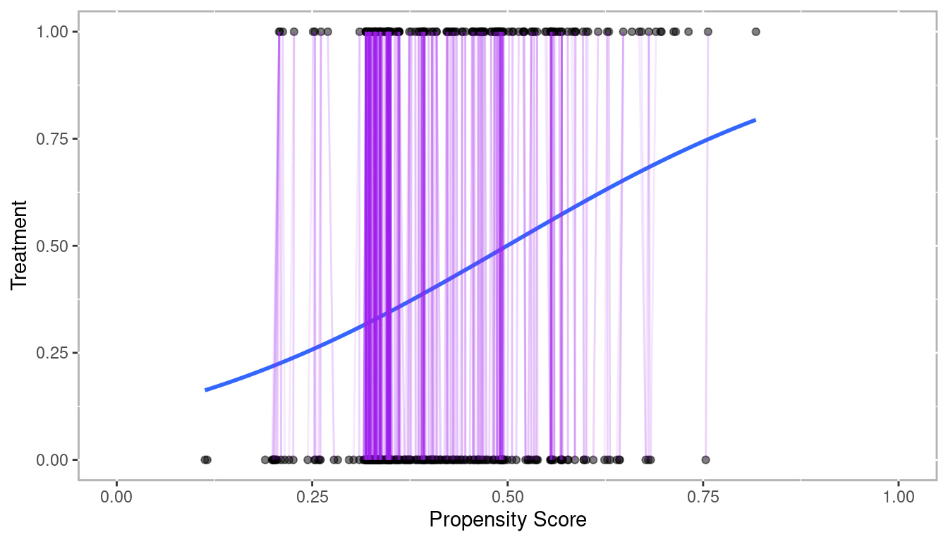
Figure 3.1: Propensity Scores from Logistic Regression with Sample of Matched Pairs
3.1 One-to-One Matching ATE
One-to-one matching with replacement (the M = 1 option). Estimating the treatment effect on the treated (default is ATT).
rr_att <- Match(Y = lalonde$re78,
                Tr = lalonde$treat,
                X = lalonde$lr_ps,
                M = 1,
                estimand='ATT')
summary(rr_att) # The default estimate is ATT here
##
## Estimate... 2153.3
## AI SE...... 825.4
## T-stat..... 2.6088
## p.val...... 0.0090858
##
## Original number of observations.............. 445
## Original number of treated obs............... 185
## Matched number of observations............... 185
## Matched number of observations (unweighted). 3463.1.1 Checking Balance
rr_att_mb <- psa::MatchBalance(
    df = lalonde,
    formu = lalonde.formu,
    formu.Y = update.formula(lalonde.formu, re78 ~ .),
    index.treated = rr_att$index.treated,
    index.control = rr_att$index.control,
    tolerance = 0.25,
    M = 1,
    estimand = 'ATT')
plot(rr_att_mb)
Figure 3.2: Covariate Balance Plot for Matching
# ls(rr_att_mb)
summary(rr_att_mb)
## Sample sizes and number of matches:
## Group n n.matched n.percent.matched
## Treated 185 185 1.0000000
## Control 260 173 0.6653846
## Total 445 358 0.8044944
##
## Covariate importance and t-tests for matched pairs:
## Import.Treat Import.Y Import.Total std.estimate t p.value
## I(educ^2) 1.931 1.5228 3.453 -0.04903 -0.8916 0.3732
## educ 2.099 1.2121 3.311 -0.05483 -0.9577 0.3389
## black 0.705 1.8424 2.547 -0.02326 -0.5383 0.5907
## I(re74^2) 0.353 1.6415 1.994 0.07581 2.0955 0.0369
## u75 0.852 0.9435 1.796 -0.06655 -1.8144 0.0705
## hisp 1.731 0.0404 1.771 0.02042 0.8161 0.4150
## nodegr 1.090 0.5011 1.591 0.03496 1.0914 0.2759
## re74 0.280 1.1019 1.382 0.07979 1.7483 0.0813
## re75 0.642 0.5903 1.232 0.06147 1.3171 0.1887
## age 0.237 0.6729 0.910 0.00896 0.1374 0.8908
## married 0.646 0.1406 0.787 0.04627 1.0000 0.3180
## I(re75^2) 0.390 0.3817 0.772 0.05125 1.0364 0.3007
## I(age^2) 0.232 0.5096 0.742 0.00297 0.0438 0.9651
## u74 0.184 0.0702 0.254 0.03913 0.7495 0.4541
## ci.min ci.max PercentMatched
## I(educ^2) -0.15719 0.05913 60.4
## educ -0.16744 0.05778 60.1
## black -0.10826 0.06173 91.0
## I(re74^2) 0.00465 0.14696 86.7
## u75 -0.13870 0.00559 89.3
## hisp -0.02879 0.06963 98.3
## nodegr -0.02804 0.09797 93.9
## re74 -0.00998 0.16956 77.2
## re75 -0.03032 0.15326 78.0
## age -0.11922 0.13713 44.8
## married -0.04474 0.13728 89.6
## I(re75^2) -0.04602 0.14852 88.7
## I(age^2) -0.13062 0.13656 49.7
## u74 -0.06356 0.14183 81.53.2 One-to-One matching (ATT)
rr.ate <- Match(Y = lalonde$re78,
                Tr = lalonde$treat,
                X = lalonde$lr_ps,
                M = 1,
                estimand = 'ATE')
summary(rr.ate)
##
## Estimate... 2013.3
## AI SE...... 817.76
## T-stat..... 2.4619
## p.val...... 0.013819
##
## Original number of observations.............. 445
## Original number of treated obs............... 185
## Matched number of observations............... 445
## Matched number of observations (unweighted). 7563.3 One-to-Many Matching (ATT)
rr2 <- Match(Y = lalonde$re78,
             Tr = lalonde$treat,
             X = lalonde$lr_ps,
             M = 1,
             ties = TRUE,
             replace = TRUE,
             estimand = 'ATT')
summary(rr2) # The default estimate is ATT here
##
## Estimate... 2153.3
## AI SE...... 825.4
## T-stat..... 2.6088
## p.val...... 0.0090858
##
## Original number of observations.............. 445
## Original number of treated obs............... 185
## Matched number of observations............... 185
## Matched number of observations (unweighted). 346
3.4 The MatchIt Package
##
## Call:
## MatchIt::matchit(formula = lalonde.formu, data = lalonde)
##
## Summary of Balance for All Data:
##           Means Treated Means Control Std. Mean Diff. Var. Ratio eCDF Mean
## distance         0.4468        0.3936          0.4533     1.2101    0.1340
## age             25.8162       25.0538          0.1066     1.0278    0.0254
## I(age^2)       717.3946      677.3154          0.0929     1.0115    0.0254
## educ            10.3459       10.0885          0.1281     1.5513    0.0287
## I(educ^2)      111.0595      104.3731          0.1701     1.6625    0.0287
## black            0.8432        0.8269          0.0449          .    0.0163
## hisp             0.0595        0.1077         -0.2040          .    0.0482
## married          0.1892        0.1538          0.0902          .    0.0353
## nodegr           0.7081        0.8346         -0.2783          .    0.1265
## re74          2095.5740     2107.0268         -0.0023     0.7381    0.0192
## I(re74^2) 28141433.9907 36667413.1577         -0.0747     0.5038    0.0192
## re75          1532.0556     1266.9092          0.0824     1.0763    0.0508
## I(re75^2) 12654752.6909 11196530.0057          0.0260     1.4609    0.0508
## u74              0.7081        0.7500         -0.0921          .    0.0419
## u75              0.6000        0.6846         -0.1727          .    0.0846
##           eCDF Max
## distance    0.2244
## age         0.0652
## I(age^2)    0.0652
## educ        0.1265
## I(educ^2)   0.1265
## black       0.0163
## hisp        0.0482
## married     0.0353
## nodegr      0.1265
## re74        0.0471
## I(re74^2)   0.0471
## re75        0.1075
## I(re75^2)   0.1075
## u74         0.0419
## u75         0.0846
##
## Summary of Balance for Matched Data:
##           Means Treated Means Control Std. Mean Diff. Var. Ratio eCDF Mean
## distance         0.4468        0.4284          0.1571     1.3077    0.0387
## age             25.8162       25.1351          0.0952     1.1734    0.0243
## I(age^2)       717.3946      675.1676          0.0979     1.1512    0.0243
## educ            10.3459       10.2649          0.0403     1.2869    0.0174
## I(educ^2)      111.0595      108.4919          0.0653     1.3938    0.0174
## black            0.8432        0.8486         -0.0149          .    0.0054
## hisp             0.0595        0.0703         -0.0457          .    0.0108
## married          0.1892        0.1892          0.0000          .    0.0000
## nodegr           0.7081        0.7676         -0.1308          .    0.0595
## re74          2095.5740     1741.2109          0.0725     1.5797    0.0146
## I(re74^2) 28141433.9907 18066538.6428          0.0883     3.5436    0.0146
## re75          1532.0556     1314.8073          0.0675     1.3933    0.0264
## I(re75^2) 12654752.6909  9126579.7979          0.0630     3.4873    0.0264
## u74              0.7081        0.7243         -0.0357          .    0.0162
## u75              0.6000        0.6108         -0.0221          .    0.0108
##           eCDF Max Std. Pair Dist.
## distance    0.1189          0.1585
## age         0.0541          0.8159
## I(age^2)    0.0541          0.7701
## educ        0.0595          0.7662
## I(educ^2)   0.0595          0.7604
## black       0.0054          0.5798
## hisp        0.0108          0.2286
## married     0.0000          0.2378
## nodegr      0.0595          0.5588
## re74        0.0432          0.6080
## I(re74^2)   0.0432          0.3620
## re75        0.0649          0.7292
## I(re75^2)   0.0649          0.3690
## u74         0.0162          0.7728
## u75         0.0108          0.7282
##
## Sample Sizes:
##           Control Treated
## All           260     185
## Matched       185     185
## Unmatched      75       0
## Discarded       0       0
# Same as above but calculate average treatment effect
rr.ate <- Match(Y = lalonde$re78,
                Tr = lalonde$treat,
                X = lalonde$lr_ps,
                M = 1,
                ties = FALSE,
                replace = FALSE,
                estimand='ATE')
summary(rr.ate) # Here the estimate is ATE
##
## Estimate... 2130.3
## SE......... 496.24
## T-stat..... 4.2929
## p.val...... 1.7638e-05
##
## Original number of observations.............. 445
## Original number of treated obs............... 185
## Matched number of observations............... 370
## Matched number of observations (unweighted). 370
## Genetic Matching
rr.gen <- GenMatch(Tr = lalonde$treat,
                   X = lalonde$lr_ps,
                   BalanceMatrix = lalonde[,all.vars(lalonde.formu)[-1]],
                   estimand = 'ATE',
                   M = 1,
                   pop.size = 16,
                   print.level = 0)
rr.gen.mout <- Match(Y = lalonde$re78,
                     Tr = lalonde$treat,
                     X = lalonde$lr_ps,
                     estimand = 'ATE',
                     Weight.matrix = rr.gen)
summary(rr.gen.mout)
##
## Estimate... 2159
## AI SE...... 814.91
## T-stat..... 2.6494
## p.val...... 0.0080631
##
## Original number of observations.............. 445
## Original number of treated obs............... 185
## Matched number of observations............... 445
## Matched number of observations (unweighted). 650
## Partial exact matching
rr2 <- Matchby(Y = lalonde$re78,
               Tr = lalonde$treat,
               X = lalonde$lr_ps,
               by = factor(lalonde$nodegr),
               print.level = 0)
summary(rr2)
##
## Estimate... 2333.2
## SE......... 682.81
## T-stat..... 3.417
## p.val...... 0.00063307
##
## Original number of observations.............. 445
## Original number of treated obs............... 185
## Matched number of observations............... 185
## Matched number of observations (unweighted). 185
## Partial exact matching on two covariates
rr3 <- Matchby(Y = lalonde$re78,
               Tr = lalonde$treat,
               X = lalonde$lr_ps,
               by = lalonde[,c('nodegr','married')],
               print.level = 0)
summary(rr3)
##
## Estimate... 1961.7
## SE......... 701.93
## T-stat..... 2.7947
## p.val...... 0.0051952
##
## Original number of observations.............. 445
## Original number of treated obs............... 185
## Matched number of observations............... 185
## Matched number of observations (unweighted). 185