4 Weighting
weight
verb
1. hold (something) down by placing a heavy object on top of it.
2. attach importance or value to.
Propensity score weighting is the approach to using propensity scores as weights in other statistical models such as regression or ANOVA. Like stratification (see Chapter 2), propensity score weighting has the advantage of all observations. In section 1.3.2 we introduced four different treatment estimators. The histograms used to conceptually explain what observations are included, or not included, in their calculation used propensity score weights. In this chapter will discuss the mathematical details of how those weights are calculated and applied, include the R code to generate the estimates.
We will present a formula for each of the treatment effects we wish to estimate. These formulas define the weights. Once we have the weights we can use them in a statistical model or using the following formula to estimate the treatment effect.
\[\begin{equation} \begin{aligned} Treatment\ Effect = \frac{\sum Y_{i}Z_{i}w_{i}}{\sum Z_{i} w_{i}} - \frac{\sum Y_{i}(1 - Z_{i}) w_{i}}{\sum (1 - Z_{i}) w_{i} } \end{aligned} \tag{4.1} \end{equation}\]
For equation (4.1), \(w\) is the weight (as defined in the following sections), \(Z_i\) is the treatment assignment such that \(Z = 1\) is treatment and \(Z = 0\) is control, and \(Y_i\) is the outcome.
4.1 Estimate Propensity Scores
To begin, we estimate the propensity scores, here using logistic regression.
4.2 Checking Balance
Checking balance for propensity score weighting is the same as stratification. Figure 4.1 is a multiple covariate balance assessment plot. See section 2.1.2 in the stratification chapter for more details on how you can check for balance for individual covariates.
PSAgraphics::cv.bal.psa(covariates = lalonde[,all.vars(lalonde.formu)[-1]],
                        treatment = lalonde$treat,
                        propensity = lalonde$lr_ps,
                        strata = 5)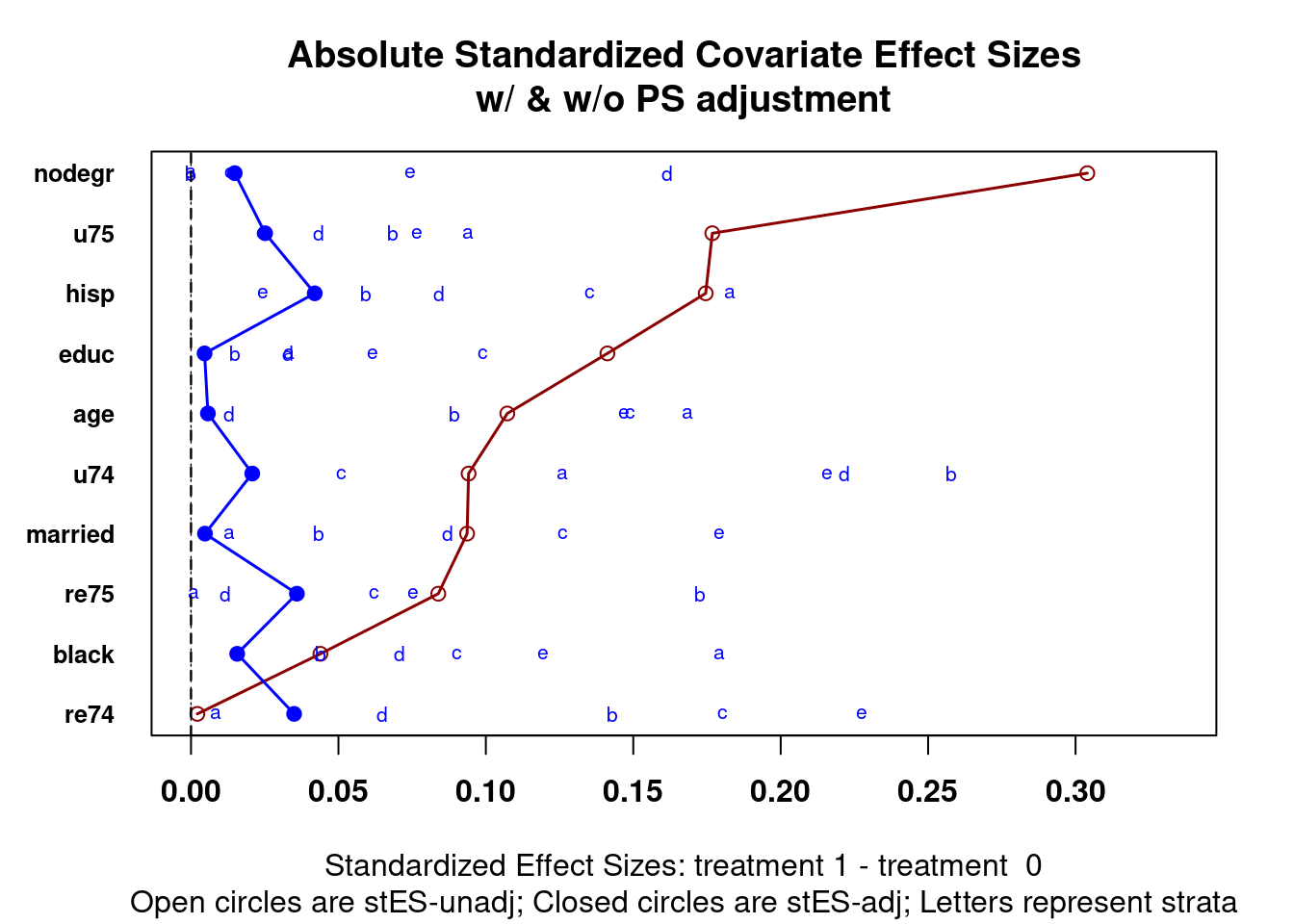
Figure 4.1: Multiple covariate balance assessment plot for Lalonde data after estimating propensity scores with logistic regression
There is one additional balance check that can be done with propensity score weights. We can run the propensity score estimation model with the estimated propensity score weights. This should result in all the covariates having a non-statistically significant effect on the treatment. We will explore the details for the four treatment effects discussed in the next section.
4.3 Average Treatment Effect (ATE)
\[\begin{equation} \begin{aligned} w_{ATE} = \frac{Z_i}{\pi_i} + \frac{1 - Z_i}{1 - \pi_i} \end{aligned} \tag{4.2} \end{equation}\]
ate_weights <- psa::calculate_ps_weights(treatment = lalonde$treat,
                                         ps = lalonde$lr_ps,
                                         estimand = 'ATE')
4.3.1 Check Balance with ATE Weights
glm(formula = lalonde.formu,
    data = lalonde,
    family = quasibinomial(link = 'logit'),
    weights = ate_weights
) |> summary()
##
## Call:
## glm(formula = lalonde.formu, family = quasibinomial(link = "logit"),
## data = lalonde, weights = ate_weights)
##
## Coefficients:
## Estimate Std. Error t value Pr(>|t|)
## (Intercept) -2.000e-01 1.977e+00 -0.101 0.919
## age 2.686e-02 8.513e-02 0.316 0.753
## I(age^2) -4.695e-04 1.397e-03 -0.336 0.737
## educ -6.326e-02 4.024e-01 -0.157 0.875
## I(educ^2) 3.510e-03 2.259e-02 0.155 0.877
## black -3.695e-03 3.714e-01 -0.010 0.992
## hisp 2.232e-02 4.904e-01 0.046 0.964
## married -8.664e-03 2.784e-01 -0.031 0.975
## nodegr 4.154e-02 3.889e-01 0.107 0.915
## re74 2.291e-05 7.493e-05 0.306 0.760
## I(re74^2) -9.734e-10 2.337e-09 -0.416 0.677
## re75 5.001e-06 1.015e-04 0.049 0.961
## I(re75^2) -3.543e-10 5.032e-09 -0.070 0.944
## u74 8.163e-02 4.449e-01 0.183 0.854
## u75 -4.153e-04 3.566e-01 -0.001 0.999
##
## (Dispersion parameter for quasibinomial family taken to be 2.067727)
##
## Null deviance: 1232.6 on 444 degrees of freedom
## Residual deviance: 1231.9 on 430 degrees of freedom
## AIC: NA
##
## Number of Fisher Scoring iterations: 44.3.2 Estimate ATE
##
## Call:
## lm(formula = re78 ~ treat, data = lalonde, weights = ate_weights)
##
## Weighted Residuals:
##
## Coefficients:
##             Estimate Std. Error t value Pr(>|t|)
## (Intercept)     4556        450  10.125   <2e-16 ***
## treat           1558        637   2.446   0.0148 *
## ---
## Signif. codes:  0 '***' 0.001 '**' 0.01 '*' 0.05 '.' 0.1 ' ' 1
##
## Residual standard error: 9497 on 443 degrees of freedom
## Multiple R-squared:  0.01333,    Adjusted R-squared:  0.0111
## F-statistic: 5.983 on 1 and 443 DF,  p-value: 0.01483
psa::treatment_effect(treatment = lalonde$treat,
                      outcome = lalonde$re78,
                      weights = ate_weights)
## 1558.094.4 Average Treatment Effect Among the Treated (ATT)
\[\begin{equation} \begin{aligned} w_{ATT} = \frac{\pi_i Z_i}{\pi_i} + \frac{\pi_i (1 - Z_i)}{1 - \pi_i} \end{aligned} \tag{4.3} \end{equation}\]
att_weights <- psa::calculate_ps_weights(treatment = lalonde$treat,
                                         ps = lalonde$lr_ps,
                                         estimand = 'ATT')
4.4.1 Check Balance with ATT Weights
glm(formula = lalonde.formu,
    data = lalonde,
    family = quasibinomial(link = 'logit'),
    weights = att_weights
) |> summary()
##
## Call:
## glm(formula = lalonde.formu, family = quasibinomial(link = "logit"),
## data = lalonde, weights = att_weights)
##
## Coefficients:
## Estimate Std. Error t value Pr(>|t|)
## (Intercept) 1.122e-01 1.754e+00 0.064 0.949
## age 2.350e-02 8.362e-02 0.281 0.779
## I(age^2) -4.382e-04 1.352e-03 -0.324 0.746
## educ -1.279e-01 3.424e-01 -0.374 0.709
## I(educ^2) 7.725e-03 1.931e-02 0.400 0.689
## black -5.090e-02 3.388e-01 -0.150 0.881
## hisp -7.925e-02 5.202e-01 -0.152 0.879
## married -2.667e-02 2.691e-01 -0.099 0.921
## nodegr 1.449e-01 3.623e-01 0.400 0.689
## re74 9.327e-06 7.444e-05 0.125 0.900
## I(re74^2) -9.597e-11 2.521e-09 -0.038 0.970
## re75 -1.340e-05 9.575e-05 -0.140 0.889
## I(re75^2) 7.444e-10 4.817e-09 0.155 0.877
## u74 -6.362e-02 4.320e-01 -0.147 0.883
## u75 8.469e-02 3.390e-01 0.250 0.803
##
## (Dispersion parameter for quasibinomial family taken to be 0.8614842)
##
## Null deviance: 513.54 on 444 degrees of freedom
## Residual deviance: 513.06 on 430 degrees of freedom
## AIC: NA
##
## Number of Fisher Scoring iterations: 44.4.2 Estimate ATT
##
## Call:
## lm(formula = re78 ~ treat, data = lalonde, weights = att_weights)
##
## Weighted Residuals:
##
## Coefficients:
##             Estimate Std. Error t value Pr(>|t|)
## (Intercept)   4557.4      454.2  10.033  < 2e-16 ***
## treat         1791.7      642.8   2.787  0.00554 **
## ---
## Signif. codes:  0 '***' 0.001 '**' 0.01 '*' 0.05 '.' 0.1 ' ' 1
##
## Residual standard error: 6186 on 443 degrees of freedom
## Multiple R-squared:  0.01724,    Adjusted R-squared:  0.01502
## F-statistic:  7.77 on 1 and 443 DF,  p-value: 0.00554
psa::treatment_effect(treatment = lalonde$treat,
                      outcome = lalonde$re78,
                      weights = att_weights)
## 1791.724.5 Average Treatment Effect Among the Control (ATC)
\[\begin{equation} \begin{aligned} w_{ATC} = \frac{(1 - \pi_i) Z_i}{\pi_i} + \frac{(1 - e_i)(1 - Z_i)}{1 - \pi_i} \end{aligned} \tag{4.4} \end{equation}\]
atc_weights <- psa::calculate_ps_weights(treatment = lalonde$treat,
                                         ps = lalonde$lr_ps,
                                         estimand = 'ATC')
4.5.1 Check Balance with ATC Weights
glm(formula = lalonde.formu,
    data = lalonde,
    family = quasibinomial(link = 'logit'),
    weights = atc_weights
) |> summary()
##
## Call:
## glm(formula = lalonde.formu, family = quasibinomial(link = "logit"),
## data = lalonde, weights = atc_weights)
##
## Coefficients:
## Estimate Std. Error t value Pr(>|t|)
## (Intercept) -6.598e-01 2.390e+00 -0.276 0.783
## age 3.097e-02 8.728e-02 0.355 0.723
## I(age^2) -5.201e-04 1.449e-03 -0.359 0.720
## educ 4.722e-02 4.975e-01 0.095 0.924
## I(educ^2) -3.225e-03 2.766e-02 -0.117 0.907
## black 3.598e-02 4.033e-01 0.089 0.929
## hisp 7.912e-02 4.941e-01 0.160 0.873
## married 7.290e-03 2.868e-01 0.025 0.980
## nodegr -7.488e-02 4.205e-01 -0.178 0.859
## re74 2.763e-05 7.658e-05 0.361 0.718
## I(re74^2) -1.296e-09 2.319e-09 -0.559 0.577
## re75 2.037e-05 1.073e-04 0.190 0.849
## I(re75^2) -1.341e-09 5.282e-09 -0.254 0.800
## u74 1.831e-01 4.577e-01 0.400 0.689
## u75 -7.234e-02 3.730e-01 -0.194 0.846
##
## (Dispersion parameter for quasibinomial family taken to be 1.206136)
##
## Null deviance: 719.09 on 444 degrees of freedom
## Residual deviance: 717.84 on 430 degrees of freedom
## AIC: NA
##
## Number of Fisher Scoring iterations: 44.5.2 Estimate ATC
##
## Call:
## lm(formula = re78 ~ treat, data = lalonde, weights = atc_weights)
##
## Weighted Residuals:
##
## Coefficients:
##             Estimate Std. Error t value Pr(>|t|)
## (Intercept)   4554.8      446.8  10.195   <2e-16 ***
## treat         1391.0      632.6   2.199   0.0284 *
## ---
## Signif. codes:  0 '***' 0.001 '**' 0.01 '*' 0.05 '.' 0.1 ' ' 1
##
## Residual standard error: 7204 on 443 degrees of freedom
## Multiple R-squared:  0.0108, Adjusted R-squared:  0.008564
## F-statistic: 4.835 on 1 and 443 DF,  p-value: 0.0284
psa::treatment_effect(treatment = lalonde$treat,
                      outcome = lalonde$re78,
                      weights = atc_weights)
## 1391.024.6 Average Treatment Effect Among the Evenly Matched (ATM)
\[\begin{equation} \begin{aligned} w_{ATM} = \frac{min\{\pi_i, 1 - \pi_i\}}{Z_i \pi_i (1 - Z_i)(1 - \pi_i)} \end{aligned} \tag{4.5} \end{equation}\]
atm_weights <- psa::calculate_ps_weights(treatment = lalonde$treat,
                                         ps = lalonde$lr_ps,
                                         estimand = 'ATM')
4.6.1 Check Balance with ATM Weights
glm(formula = lalonde.formu,
    data = lalonde,
    family = quasibinomial(link = 'logit'),
    weights = atm_weights
) |> summary()
##
## Call:
## glm(formula = lalonde.formu, family = quasibinomial(link = "logit"),
## data = lalonde, weights = atm_weights)
##
## Coefficients:
## Estimate Std. Error t value Pr(>|t|)
## (Intercept) 1.657e-01 2.129e+00 0.078 0.938
## age -2.418e-02 8.893e-02 -0.272 0.786
## I(age^2) 4.192e-04 1.465e-03 0.286 0.775
## educ 6.308e-02 4.304e-01 0.147 0.884
## I(educ^2) -3.347e-03 2.420e-02 -0.138 0.890
## black 1.480e-02 3.577e-01 0.041 0.967
## hisp -3.495e-02 5.203e-01 -0.067 0.946
## married -3.486e-03 2.736e-01 -0.013 0.990
## nodegr -4.659e-02 3.825e-01 -0.122 0.903
## re74 -2.333e-05 7.526e-05 -0.310 0.757
## I(re74^2) 8.298e-10 2.510e-09 0.331 0.741
## re75 -7.419e-06 9.758e-05 -0.076 0.939
## I(re75^2) 7.957e-10 4.775e-09 0.167 0.868
## u74 -6.630e-02 4.360e-01 -0.152 0.879
## u75 -3.051e-02 3.436e-01 -0.089 0.929
##
## (Dispersion parameter for quasibinomial family taken to be 0.7850194)
##
## Null deviance: 467.94 on 444 degrees of freedom
## Residual deviance: 467.73 on 430 degrees of freedom
## AIC: NA
##
## Number of Fisher Scoring iterations: 34.6.2 Estimate ATM
##
## Call:
## lm(formula = re78 ~ treat, data = lalonde, weights = atm_weights)
##
## Weighted Residuals:
##
## Coefficients:
##             Estimate Std. Error t value Pr(>|t|)
## (Intercept)   4504.6      459.8   9.797  < 2e-16 ***
## treat         1707.7      648.8   2.632  0.00878 **
## ---
## Signif. codes:  0 '***' 0.001 '**' 0.01 '*' 0.05 '.' 0.1 ' ' 1
##
## Residual standard error: 5960 on 443 degrees of freedom
## Multiple R-squared:  0.0154, Adjusted R-squared:  0.01318
## F-statistic: 6.928 on 1 and 443 DF,  p-value: 0.008783
psa::treatment_effect(treatment = lalonde$treat,
                      outcome = lalonde$re78,
                      weights = atm_weights)
## 1707.69